Permutation Tests

Nearly bomb-proof tests for arbitrary distributions and measurements

Author

Trent McDonald

Published

July 10, 2023

Permutation tests are powerful, almost bomb-proof, multi-sample statistical tests. Permutation tests are not widely taught, and most internet pages on the subject are complicated and specialized. I explain and demonstrate permutation tests in R and hope non-statisticians adopt them as default tests.

Background

Permutation tests are similar to and accomplish the same thing as t-tests and F-tests. All these methods, and others, test for statistical differences among two or more samples. I focus on the two sample case for simplicity even though permutation tests apply to three or more samples. The primary difference between the parametric tests (e.g., the t test) and permutation tests is that permutation tests are non-parametric and do not assume data arise from a particular theoretical distribution.

Permutation Tests

Suppose we obtain twelve values of some measurement on twelve subjects, six randomly selected from one group and six randomly selected from another. Equality of sample sizes does not matter. Perhaps we have four measured heights for men in a particular group (say, seniors in a high school) and six height measurements for women in the same group. Perhaps we have ten estimates of fish biomass in a particular lake during 2021 and seven measurements of the same thing in 2022.

The following R code loads an example data set with 6 and 6 values in each sample. For clarity, the example data is listed in Table 1 and plotted in Figure 1.

s1 <- c( 0.0, 0.301, 0.602, 1.58, 1.96, 2.33) 
s2 <- c( 0.0, 0.0  , 0.0  , 1.51, 1.78, 1.78)
n1 <- length(s1)
n2 <- length(s2)
exDf <- data.frame(
  sample = c(rep("Sample 1", n1), rep("Sample 2", n2))
  , x = c(s1, s2)
)

Table 1: Two samples of a measurement on twelve subjects, six in each sample.

sample	x
Sample 1	0.000
Sample 1	0.301
Sample 1	0.602
Sample 1	1.580
Sample 1	1.960
Sample 1	2.330
Sample 2	0.000
Sample 2	0.000
Sample 2	0.000
Sample 2	1.510
Sample 2	1.780
Sample 2	1.780

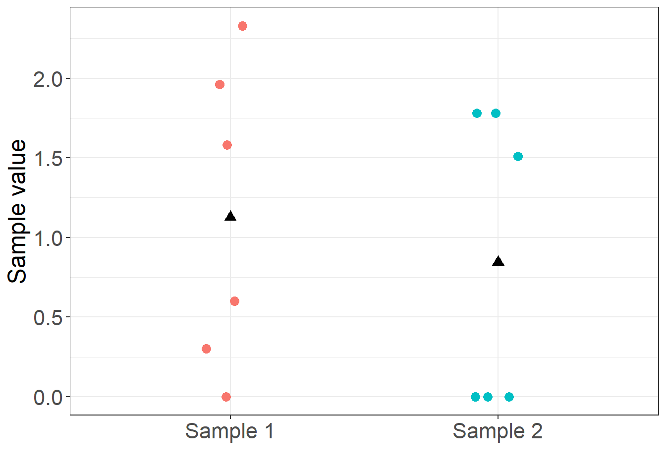
Figure 1: A plot of values used in the example. Values have been jittered horizontally to show overlapping points. Black triangles are the sample means.

The question is whether the mean of the random process that generated sample 1 is different from the mean of the random process that generated sample 2. Is the mean of sample 1 equal to the mean of sample 2? In statistical notation, we wish to test the null hypothesis, $H_{0} : μ_{1} = μ_{2}$ against the alternative, $H_{A} : μ_{1} \neq μ_{2} .$

Technically,

H_{0}

involves the entire distribution

Technically, permutation methods test for any different in the underlying distributions. Technically, the correct null hypothesis is $H_{0} : F_{1} = F_{2}$ , where $F_{i}$ is the entire distribution from which sample $i$ was drawn. This means that permutation tests are sensitive to differences in quantiles which implies the distributions differ in location, shape, or both. For simplicity, and because it is the most popular case, and because a difference in means is a difference in location, I frame the hypothesis as equality of means.

Permutation tests reason that if the null hypothesis is true, values that ended up in sample 1 could just as easily have ended up in sample 2, and vice versa. In other words, if $H_{0}$ is true the behind-the-scenes assignment of values to samples was completely random and the labels “Sample 1” and “Sample 2” mean nothing. If labels mean nothing, we can randomly reassign them and the resulting difference in means is just a random observation of how much the means could differ if the underlying distributions are equal.

That is the heart of the permutation reasoning. If we randomly permute the values among samples many times, we can build the entire distribution of the test statistic when the null hypothesis is true. If the original difference in means computed on un-permuted values is unlikely to have come from this distribution, the null hypothesis must be wrong. If the original mean difference is typical of the mean differences we would see if the null hypothesis is true, we conclude that the null hypothesis could be true. We usually set “unlikely” to mean less than 5% of the distribution is more extreme (in absolute value, assuming a two-tailed test) than the original test statistic. Conversely, we take “typical” to mean more than 5% of the distribution is more extreme than the original test statistic.

Note: Here, our test statistic is the difference in sample means ${\bar{x}}_{1} - {\bar{x}}_{2}$ . Permutation works for any test statistic. We could compute the difference in sample maximums or the ratio of two proportions.

Key justification for permutation tests

If $H_{0}$ is true, the labels “Sample 1” and “Sample 2” mean nothing. We can therefore obtain random values of the test statistic under $H_{0}$ simply by randomly assigning values to samples (or sample labels to values) and recomputing the statistic many times.

Example

I conduct a permutation test of the mean difference on the example data in Table 1. I make heavy use of the dplyr and rsample packages that are part of the so-called tidyverse of packages. Explanation of tidyverse functionality and syntax is beyond the scope of this post, except to say that these functions are un-naturally fast (kudos to their authors). It is not possible to write your own permutation code that executes faster than rsample::permutations() and dplyr::summarise(), so I encourage you to go ahead and drink the tidyverse Kool-Aid. At the same time, writing your own permutation code will illuminate the calculations and that will enhance understanding.

Here is the permutation code in R:

# Number of permutations to do
R <- 1000

# A function to compute mean difference on one permutation
# Result is mean of Sample 2 minus Sample 1. 
meanDiff <- function(permedDf, key){
  permedDf[[1]] %>% 
    rsample::analysis() %>%
    dplyr::group_by(sample) %>% 
    dplyr::summarise(xbar = mean(x)) %>% 
    dplyr::ungroup() %>% 
    dplyr::summarise(xbarDiff = diff(xbar))  %>% 
    dplyr::pull(xbarDiff)
}

# Use rsample package to do the permutations 
perms <- exDf %>% 
  rsample::permutations(x, times = R, apparent = TRUE)

# dataset 'perms' contains one row of lists 
# per permutation, and one for the original
nrow(perms)

[1] 1001

tail(perms)

# A tibble: 6 × 2
  splits          id              
  <list>          <chr>           
1 <split [12/0]>  Permutations0996
2 <split [12/0]>  Permutations0997
3 <split [12/0]>  Permutations0998
4 <split [12/0]>  Permutations0999
5 <split [12/0]>  Permutations1000
6 <split [12/12]> Apparent

# Examine a permutation to make sure rsample is working right
# Confirm that every value in original appears once
(perms$splits[[1]] %>% rsample::analysis())

     sample     x
1  Sample 1 0.000
2  Sample 1 1.780
3  Sample 1 0.000
4  Sample 1 0.301
5  Sample 1 1.780
6  Sample 1 2.330
7  Sample 2 0.000
8  Sample 2 1.580
9  Sample 2 1.960
10 Sample 2 0.602
11 Sample 2 0.000
12 Sample 2 1.510

# The original un-permutated sample has id = "Apparent"
(perms$splits[perms$id == "Apparent"][[1]] %>% rsample::analysis())

     sample     x
1  Sample 1 0.000
2  Sample 1 0.301
3  Sample 1 0.602
4  Sample 1 1.580
5  Sample 1 1.960
6  Sample 1 2.330
7  Sample 2 0.000
8  Sample 2 0.000
9  Sample 2 0.000
10 Sample 2 1.510
11 Sample 2 1.780
12 Sample 2 1.780

# Compute the test statistic (mean difference) on all permutations
meanDiffs <- perms %>% 
  dplyr::group_by(id) %>% 
  dplyr::summarise(meanDiff = meanDiff(splits))

That’s it. The hard part is done thanks to rsample and dplyr. Data frame meanDiffs contains 1000 values of the difference in means under the null hypothesis, and it contains the original difference in means which is a legitimate observation from the null distribution if the null hypothesis is true. A total of 1001 observations. This is what the meanDiffs data frame looks like:

head(meanDiffs)

# A tibble: 6 × 2
  id               meanDiff
  <chr>               <dbl>
1 Apparent          -0.284 
2 Permutations0001  -0.0898
3 Permutations0002  -0.0105
4 Permutations0003   0.727 
5 Permutations0004   0.0172
6 Permutations0005   0.123

All that is left is to summarize the null distribution and compute the p-value. Recall from Statistics 101, the p-value of a hypothesis is the probability of obtaining a test statistic as large or larger in magnitude as the original one, if the null hypothesis is true. Assuming $x$ is our original test statistic (mean difference), computing a two-sided p-value involves computing the proportion of random test statistics less than $- | x |$ plus the proportion of random test statistics greater than $| x |$ . If the chances of seeing the original test statistic in the null distribution is low, say less than 0.05, we infer that the null hypothesis is wrong and we conclude that the underlying random mechanisms generating the two samples are different.

Before computing the p-value I like to look at the distribution of the test statistic we built using permutation. The following code does that, and produced a picture of the distribution in Figure 2.

origDiff <- meanDiffs$meanDiff[meanDiffs$id == "Apparent"]
smuDens <- density(meanDiffs$meanDiff, width = MASS::width.SJ(meanDiffs$meanDiff))
histBars <- hist(meanDiffs$meanDiff
     , n = 40
     , plot = FALSE)
hist(meanDiffs$meanDiff
     , n = 40
     , prob = T
     , main=""
     , xlab = "Mean Difference [(Sample 2) - (Sample 1)]"
     , ylim = c(0, max(histBars$density, smuDens$y)) )
lines(smuDens, col="red", lwd=3)
abline(v = c(origDiff, abs(origDiff))
       , col = "blue"
       , lwd = 3
       , lty = c(1,2))
axis(1 
     , at = round(c(origDiff, abs(origDiff)), 2)
     , col.axis = "blue"
     , line = 1
     , tick = FALSE
)

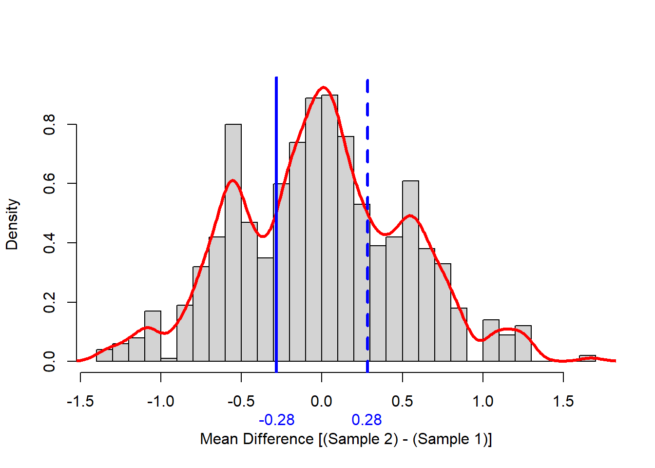
Figure 2: Histogram (grey) of the test statistic’s null distribution that we obtained by permutation. Red line is a smoothed histogram estimate. Blue vertical lines are the original mean difference (solid) and the absolute value of the original mean difference computed on un-permuted values (dashed).

Note that the null distribution is not normal, it is pretty symmetric, and it is multi-modal (has more than one hump). The minor modes (humps) were likely generated a large number of zeros in one sample or the other.

Finally, the p-value for our example null hypothesis is,

# Finally, compute two-sided p-value. 
pval <- mean( meanDiffs$meanDiff <= -abs(origDiff) | abs(origDiff) <=  meanDiffs$meanDiff )
cat(paste("The proportion of the null distribution more\nextreme than the original test statistic is", round(pval, 4), "\n"))

The proportion of the null distribution more
extreme than the original test statistic is 0.5934

Conclusion: We cannot reject the null hypothesis of equality because the p-value is well above 5%. The underlying mechanisms that generated Sample 1 and Sample 2 could be the same.

Comparison to Theory

For comparison, I overlay the regular normal-theory null distribution on the permutation distribution I obtained above. The regular normal-theory null distribution is the distribution we would have used to compute the p-value had we not performed permutation. In this case, the theoretical distribution for the difference of two means assuming equal variances is normal with variance equal to the pooled variance estimator. In other words, I plot the theoretical normal distribution for the numerator of Student’s t-ratio.

# Pooled variance of two sample t-test 
se <- sqrt( sd(exDf$x) * (1/n1 + 1/n2) ) 

# The theoretical distribution
xnorm <- seq(min(meanDiffs$meanDiff), max(meanDiffs$meanDiff), length= 500)
ynorm <- dnorm(xnorm, mean = 0, sd= se)

# Overlay plot
plot(range(xnorm, smuDens$x)
     , range(ynorm, smuDens$y)
     , type = "n"
     , xlab = "Mean Difference [(Sample 2) - (Sample 1)]"
     , ylab = "Density")

lines(smuDens, col="red", lwd=3)
lines(xnorm, ynorm, col="blue", lwd=3)
legend("topleft"
       , legend = c("Permutation based", "Theoretical")
       , title = "Null distributions:"
       , lwd = 3
       , col = c("red", "blue")
       , lty = 1)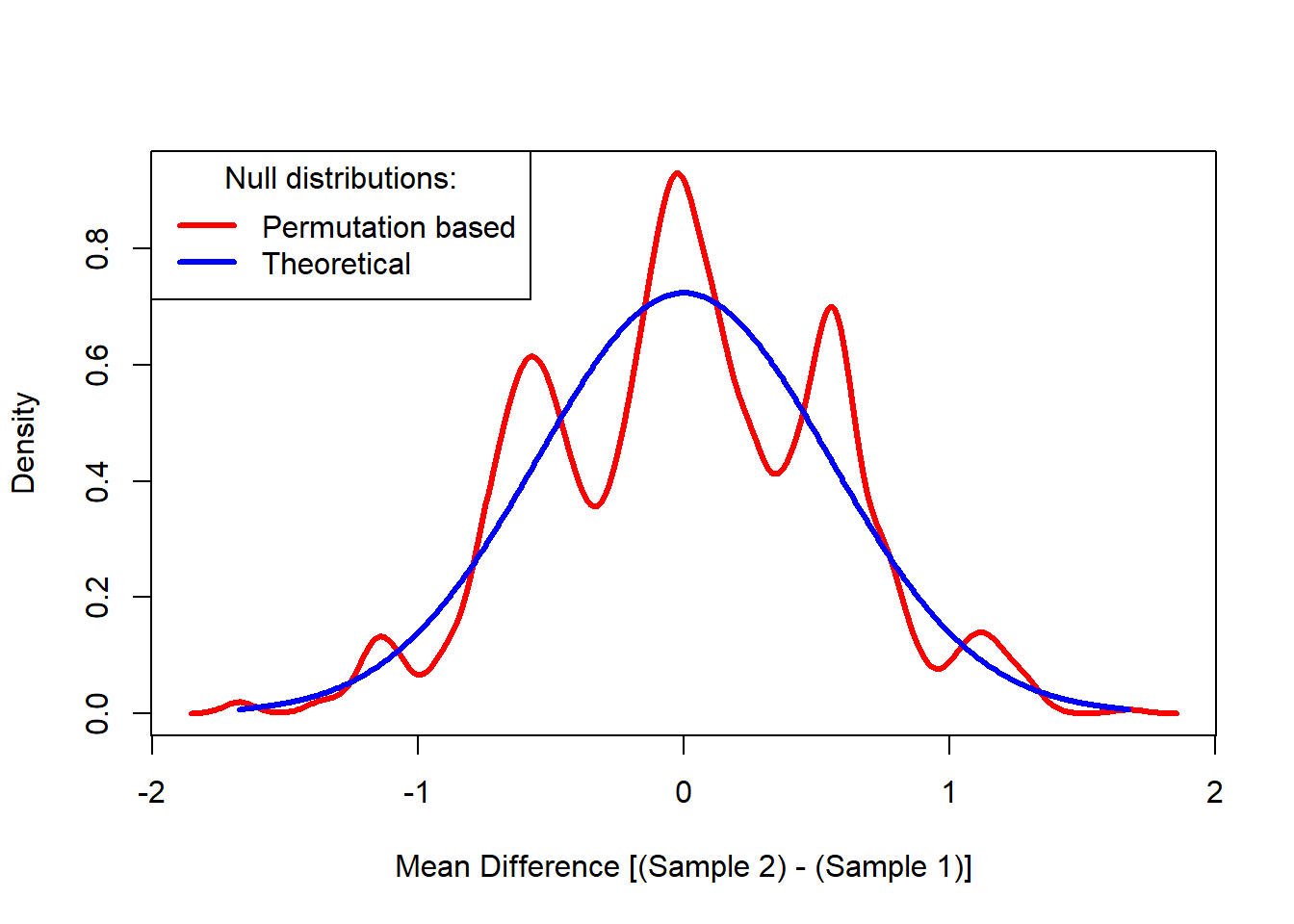

Figure 3: The permutation-based and theory-based null distributions for the example.

The p-value calculated from the theoretical (normal) distribution in this case is,

pvalNorm <- 2*pnorm(-abs(origDiff), mean = 0, sd = se) 

# The normal p-value based on theory
pvalNorm

[1] 0.6066984

# The permutation based p-value
pval

[1] 0.5934066

In our example, there are 6 values in each sample. The Central Limit Theorem is very strong and the normal approximation to the mean of 6 values is pretty good, no matter how non-normal their individual distributions are. In our example, it is not surprising that the permutation based p-value is close to the theoretical p-value based on the normal distribution.

But, before discounting permutation tests because of their proximity to normal theory tests, consider the following:

The normal-theory and permutation-based p-values may be much different in the tails because they are sensitive to numerous factors. Our example mean difference was in the heart of the null distribution where the normal-theory and permutation-based distributions won’t differ much.
The normal-theory and permutation-based p-values diverge as sample sizes become smaller.
We don’t know for sure the theoretical p-value and permutation-based p-values are close until we compute both.
The normal-theory and permutation-based p-values will differ more when other test statistics are used. The Central Limit Theorem does not apply to non-means, and it is weaker for mean-like statistics that involve subsets of the sample (e.g., extremes, proportions).
It is not possible to compute theoretical distributions of many test statistics. For example, the theoretical distributions of medians, modes, extremes, proportions, and order statistics are hard to compute.

Final Comments

Advantages

Permutation tests are better than the analogous parametric test for the following reasons:

Permutation tests make no assumptions about the underlying distribution of data in each sample.
Permutation tests can be applied to any measure of sample difference. For example, the permutation method can test for a difference in the underlying medians, maximums, or a particular percentile.
I did not discuss it here, but permutation tests are less sensitive to variance differences among samples than parametric tests. Both permutation and parametric tests are upset by differences in the underlying variances (i.e., the Behrens-Fisher problem), but permutation tests that use a properly scaled test statistic, like Student’s t ratios, are much more robust to violations of this assumption than parametric tests.

Disadvantages

I can think of two disadvantages of permutation tests:

Permutation tests require a computer and some programming to complete. Hence, they cannot be conducted in the field unless sample sizes are really small, and it takes both programming and a little execution time to compute. The permutation calculations in this post required less than 1.5 seconds to execute.
Final p-values change every time they are computed because they depend on random number sequences. To avoid this, set and save the random number seed, or run so many iterations that p-value changes are inconsequential.