multhist <- function(...
                   , bin.width
                   , col
                   , dir
                   , probability = FALSE
                   , xlab = NULL
                   , ylab = NULL
                   , main = NULL
                   , cex.lab = 1) {

  vals <- list(...)
  vrng <- range(vals)

  brks <- seq(vrng[1] - abs(diff(vrng)*0.1),
              vrng[2] + abs(diff(vrng)*0.1),
              by = bin.width)

  if(probability){
    cntOrDen <- "density"
  } else {
    cntOrDen <- "counts"
  }
  yrng <- max(sapply(lapply(vals, hist, breaks = brks, plot = FALSE), "[[", cntOrDen))
  yrng <- 1.2*c(-1*yrng, yrng)

  plot.new()
  plot.window(ylim = yrng, xlim = vrng)

  addhist <- function(x, col, dir, prob) {
    par(new = TRUE)
    hist(x = x
       , ylim = dir*yrng
       , col = col
       , xlab = ""
       , ylab = ""
       , main = ""
       , axes = FALSE
       , breaks = brks
       , probability = prob
       )
  }

  mapply(addhist
       , x = vals
       , col = col
       , dir = dir
       , prob = probability)

  py <- pretty(yrng)
  py <- py[py >= yrng[1] & py <= yrng[2]]
  axis(side = 2, at = py, labels = abs(py))
  axis(side = 1)
  title(main = main, xlab = xlab, ylab = ylab, cex.lab = cex.lab)

  invisible(1)
}Mirrored Histograms
R
Mirrored histograms are excellent for comparison of proportions. Proportion comparison is at the heart of habitat analysis and I use them often.
Mirrored Histogram Routine
I recently found a great routine on Stack Overflow that deserves amplification. The post was in response to “How to create mirrored histograms” by user dayne on 29 Apr 2015. I modified dayne’s routine slightly to allow frequency (unscaled) and probability (scaled) histograms using parameter probability, and I disabled background plotting when computing maximum bar height which produced one histogram per vector when run in RMarkdown. Here is the updated routine:
Input Parameters: The ... parameter can accept arbitrary numeric vectors. bin.width is a single bin width that will be applied to each vector. col is a vector of colors the same length as the number of vectors in .... dir is a vector containing 1 or -1 that is the same length as the number of vectors in .... Vectors corresponding to a -1 in dir are plotted downward in the mirrored histogram. Vectors corresponding to a 1 in dir are plotted upward in the figure. If probability is TRUE, all histograms are scaled to sum to 1.0. If probability is FALSE, histograms in the figure report frequencies. The remaining input parameters are standard R graphics parameters.
Examples
Examples of the figures this function produces.
Two Vector Frequency
s1 <- rnorm(50, sd = 10)
s2 <- runif(50, min=-20, max=20)
multhist(s1, s2
         , bin.width = 2
         , col = c("lightblue", "lightgreen")
         , dir = c(1,-1))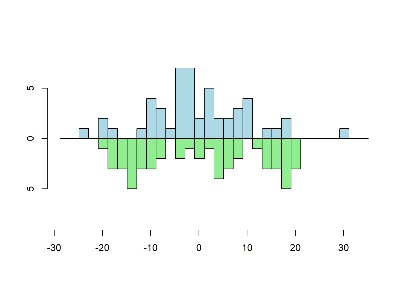
Two Vector Probability
When input vector lengths differ, probability (scaled) histograms are best for comparison because the y-axis has the same scale for both.
s1 <- rnorm(5000, sd = 10)
s2 <- runif(300, min=-20, max=20)
multhist(s1, s2
         , bin.width = 2
         , col = c("lightblue", "lightgreen")
         , dir = c(1,-1)
         , probability = TRUE
         , xlab = "Random normal and uniform"
         , ylab = "Density")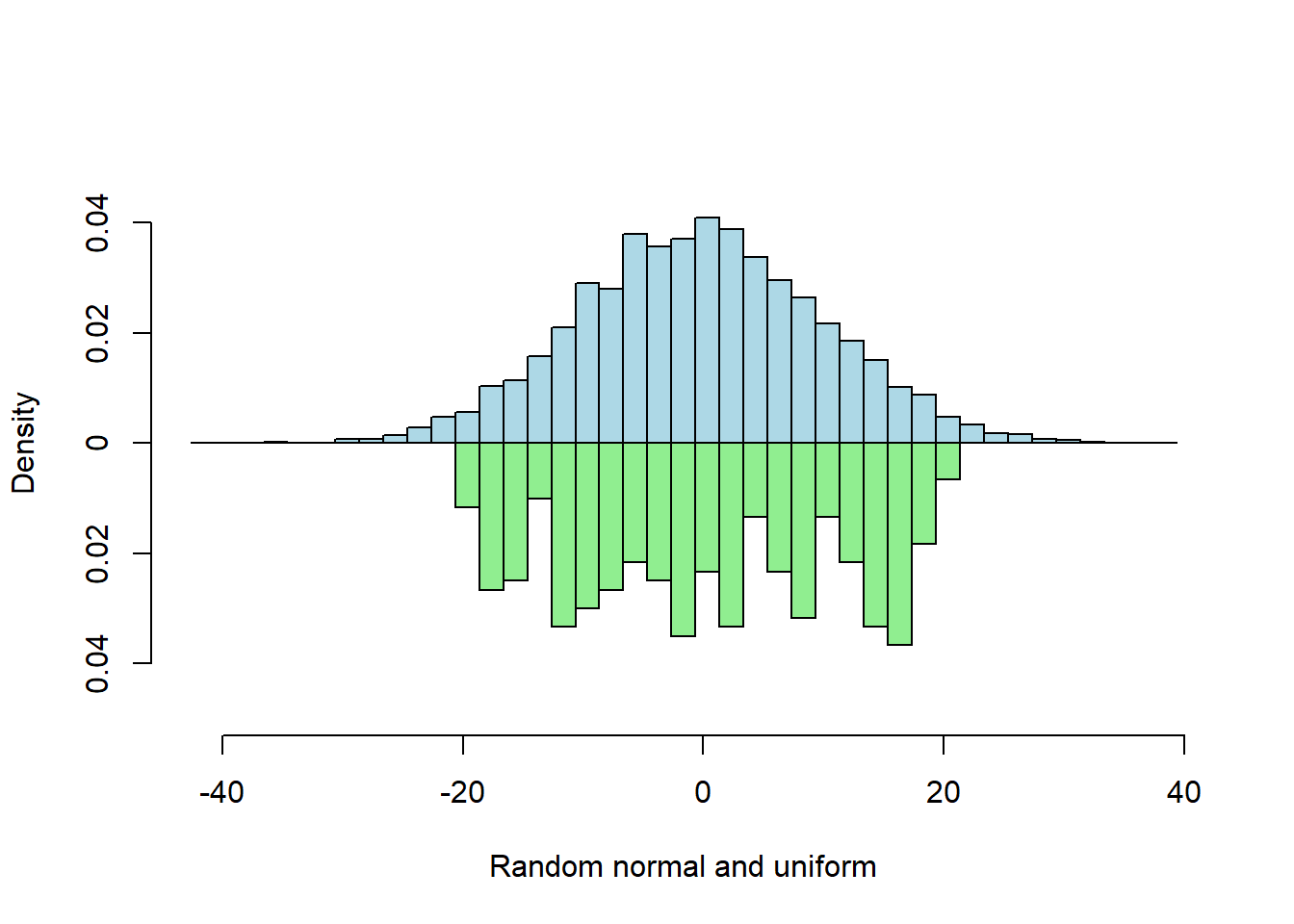
Four Vectors
s1 <- rnorm(5000, sd = 10)
s2 <- runif(300, min=-20, max=20)
s3 <- rpois(5000, 10)
s4 <- rnorm(300) * 5 - 10

multhist(s1, s2, s3, s4
         , bin.width = 2
         , col = c("lightblue", "lightgreen", "yellow", "purple")
         , dir = c(1,-1, 1, -1)
         , probability = TRUE
         , xlab = "Random normal and uniform"
         , ylab = "Density")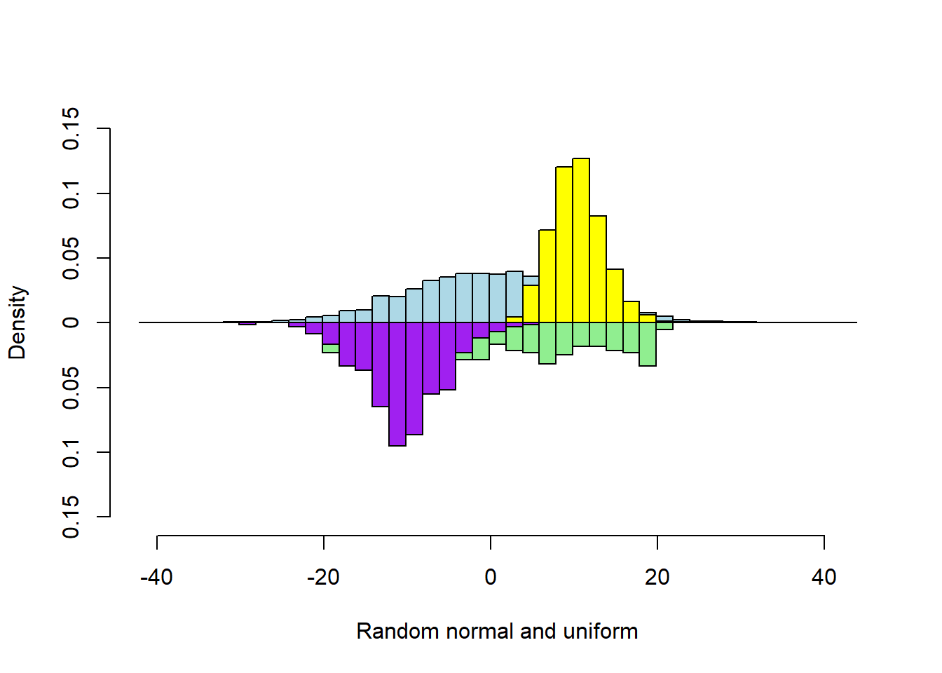
Transparency
The previous figure is good, but some bars are occluded. Judicious use of transparency reveals the occluded bar heights.
s1 <- rnorm(5000, sd = 10)
s2 <- runif(300, min=-20, max=20)
s3 <- rpois(5000, 10)
s4 <- rnorm(300) * 5 - 10

col1 <- rgb(0,.5,.2, alpha=.5)
col2 <- rgb(.5,.5,0, alpha=.5)
col3 <- rgb(1,0,0, alpha=.5)
col4 <- rgb(0,0,1, alpha=.5)

multhist(s1, s2, s3, s4
         , bin.width = 2
         , col = c(col1, col3, col2, col4)
         , dir = c(1,-1, 1, -1)
         , probability = TRUE
         , xlab = "Four distributions"
         , ylab = "Density")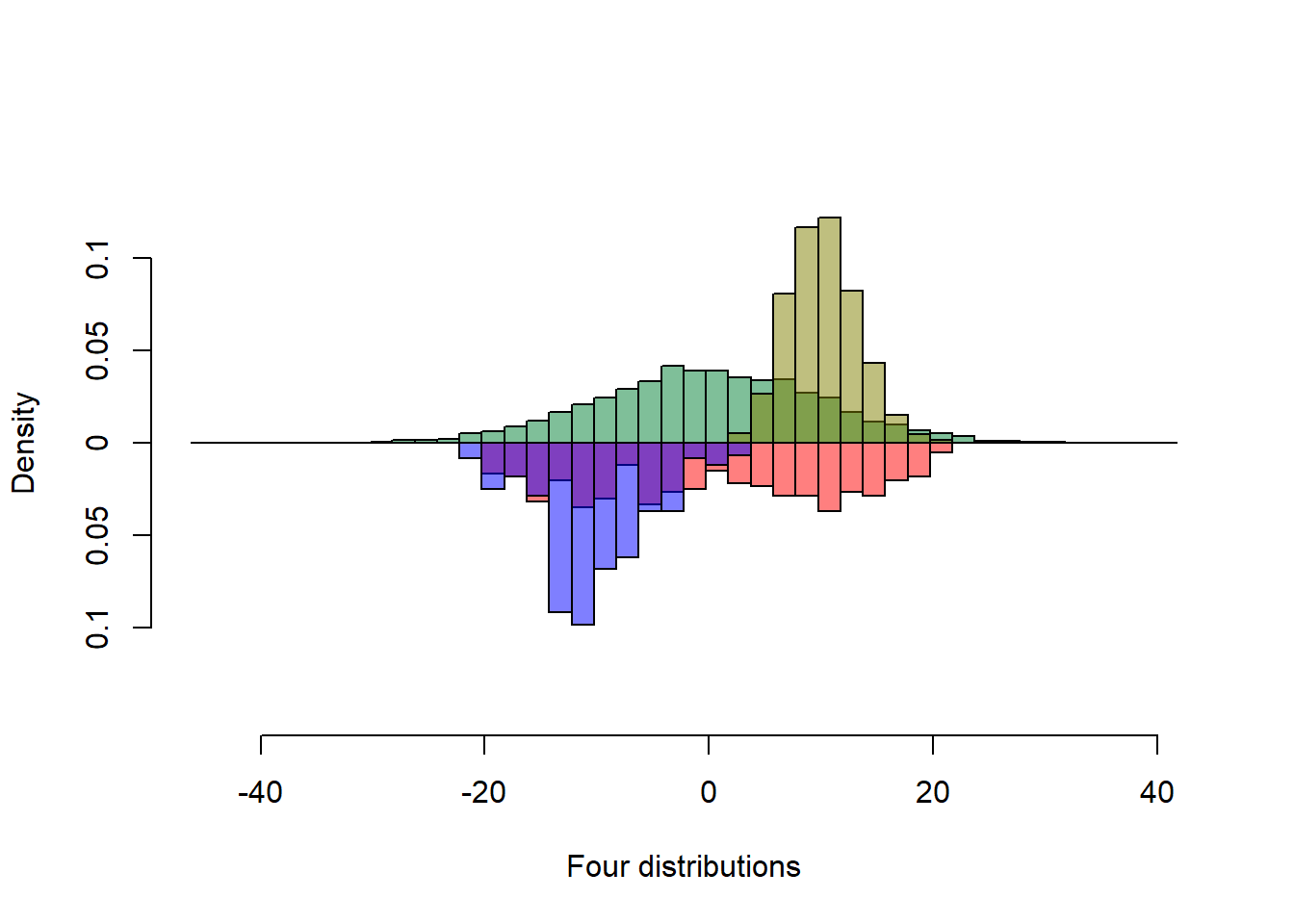
Mirrored Histograms in Habitat Analysis
In habitat analysis, one vector in the mirrored histogram is a characteristic of habitat at locations where an animal was observed. For example, the elevation of a mountain lion’s location as recorded by a satellite collar. We say this vector contains characteristics of the used locations. The other vector contains observations of the same characteristic at locations where the animal could have been. For example, the elevation of random locations in Medicine Bow National Forest. We say this vector contains characteristics of available locations.
Mirrored histograms, with the distribution of used characteristics plotted upward and the distribution of available characteristics plotted downward, reveals habitat selection. The ratios of used bar heights relative to the corresponding available bar height are the selection ratios defined by Manly et al. (2002) and others. If no preferential habitat selection is taking place, the animal is moving around at random in its landscape, the distribution of the characteristic on used locations will look like (be within random error of) the distribution of the characteristic on available locations. If selection is taking place, the used characteristic distribution will be different than the available characteristic distribution. If a bar’s height ratio is >1, selection is preferentially for locations with this characteristic in the range of the bar. If the ratio of a bar is <1, selection is against locations with characteristics in the range of the bar. Often, we actually compute the bar height ratios and plot them verses values of the characteristic. This plot, and the mirrored histogram itself, provides an good visual indicator of selection in one dimension of habitat.
There are other considerations and complexities involved in habitat analysis. For example, we need to be sure we have a random sample of used locations. It is best to be sure all locations deemed available are actually available to the animal. We need to consider more than one dimension of habitat. We often have more than one individual involved and need to consider variation across individuals. Nonetheless, mirrored histograms are a great place to start habitat analysis.
References
Manly, B. F., McDonald, L. L., Thomas, D. L., McDonald, T. L., Erickson, W. P., (2002) Resource selection by animals: statistical design and analysis for field studies 2nd edition, Kluwer Academic Publishers: Dordrecht, Netherlands