Zoom To Point

Center native R plots of spatial objects on a point, and use a specified zoom level

Spatial

Author

Trent McDonald

Published

January 4, 2024

Native R plots (using plot) are quick and easy ways to check spatial objects. Native R plots, however, are static and changing the plot extent (zooming or panning) is not possible after the plot is generated. The mapview package is a great package that allows zooming and moving after plot generation. But, I either struggle to get mapview working, mostly because I cannot remember the syntax. Consequently, I find myself plotting spatial objects using native R plots because these plots are quick, their syntax is familiar, their options for colors and symbols is extensive, and they produce elegantly simple plots for non-publish-quality reports. The only problem - native R plots are static. You cannot zoom in (easily), and this is frustrating.

In this post I describe a function that will allow the user to set a zoom level, center a plot region on a point, and create a native R plot. This function is particularly handy when spatial tasks or checks need to be automated or programmed in code. While I target native R plots built using the plot() generic function, the function is useful for setting the extent of spatial plots generated by ggplot2::ggplot(). My function is based on a related R-bloggers post by Markus Konrad. I modified the code in the “center point” portion of Markus’s post to use native R plots, and I rolled everything into a function that returns a useful value.

Note

I use the package::function syntax in R for functions that reside in non-base packages.

You will need to following R packages to reproduce results in this post:

sf, dplyr, units, rnaturalearth, and ggplot2.

Function Description

My function, zoomToPoint, takes a sfc_POINT, a zoom level (a real number $\geq$ 0), and (optionally) a sf object to plot. When the sf object is provided, zoomToPoint centers the native R plot on the point and sets the plot’s extent based on the level of zoom. If the sf object is not given, the plot’s extent (window) is returned as a sf POLYGON and can be used later to control plotting.

Parameters:

centerPt: A sfc_POINT object. The resulting plot extent will be centered on this point.
x: An optional sf object to be plotted. If given, x and centerPt must be in the same coordiante reference system (CRS).
zoomLevel: The level of zoom. Zoom levels follow the OpenStreetMap convention. Zoom level 0 shows the whole world. Zoom level 1 shows a quarter of the world map. Zoom level $i$ shows $1 / 4^{i}$ of the earth’s extent. There is no upper limit on zoom extent, but zoomLevel $\geq$ 19 produces a plot too small to be useful. zoomLevel does not need to be an integer, it can be a decimal (e.g., 3.5).

Return Value:

zoomToPoint returns a sf object containing the plot’s extent as a rectangle in the CRS of centerPt. The return can be used to control later plot extents. If x is provided (i.e., not NULL), it will be plotted, centered on centerPt, and with the specified zoom level. If x is NULL, no plotting is done.

Function `zoomToPoint`

zoomToPont’s code is as follows:

zoomToPoint <- function(centerPt
                      , x = NULL
                      , zoomLevel = 0){
    
  if( !inherits(centerPt, "sfc_POINT") ){
    stop("Object 'centerPt' must be a 'sfc_POINT' object.")
  }
  
  if( units(sf::st_crs(centerPt)$ud_unit) == units(units::set_units(1, "degree")) ){
    C <- 360
  } else if( units(sf::st_crs(centerPt)$ud_unit) == units(units::set_units(1, "m"))){
    C <- 40075016.686   # ~ circumference of Earth in meters
  } else {
    stop(paste("Unknown units in CRS."
               , "Found "
               , sf::st_crs(centerPt)$ud_unit))
  }
  
  x_span <- C / 2^zoomLevel
  y_span <- C / 2^(zoomLevel+1)
  
  ll <- sf::st_coordinates(centerPt - c(x_span, y_span) / 2)
  ur <- sf::st_coordinates(centerPt + c(x_span, y_span) / 2)
  
  zoomReal <- list(
      x = c(ll[1,1], ur[1,1])
    , y = c(ll[1,2], ur[1,2])
  )
  
  zoomPol = sf::st_sfc(
    sf::st_polygon(
      list(
        cbind(
          zoomReal$x[c(1,2,2,1,1)],
          zoomReal$y[c(1,1,2,2,1)])
      )
    )
    , crs = sf::st_crs(centerPt)
  )
  
  zoomPol <- sf::st_as_sf(zoomPol) |>
    sf::st_set_geometry("geometry")
  
  if( !is.null(x) ){
    # replot
    plot(zoomPol$geometry, border = 0)
    plot(x$geometry, add = T)
  }
  
  zoomPol
  
}

zoomToPoint checks the class of the input centerPt, which must be sfc_POINT in this version. User’s can convert other sf objects to a simple feature POINT class (i.e., to sfc_POINT) using sf::st_as_sfc(). zoomToPoint then checks the units of centerPt’s CRS. If its units are degrees, zoomToPoint assumes coordinates are latitudes and longitudes. If units are meters, zoomToPoint assumes the CRS is projected. Given this, zoomToPoint computes the plot’s extent (plotting window) based on the requested zoom level, and constructs a sf data frame containing a single rectangle covering the plot’s extent. If object x is given, the plot extent is used to plot x.

Examples

We need a large sf object to plot as an example. The following retrieves a world map object using the rnaturalearth package.

worldmap <- rnaturalearth::ne_countries(scale = 'medium'
                                        , type = 'map_units', returnclass = 'sf')

Example 1: Aruba

The following code leaves the underlying map in lat-long coordinates, centers the plot on Aruba, and sets zoom level 3.

# Compute centroid of Aruba
aruba <- sf::st_centroid(
  worldmap |> 
    dplyr::filter(name == "Aruba") |> 
    dplyr::select(geometry)
)
aruba

Simple feature collection with 1 feature and 0 fields
Geometry type: POINT
Dimension:     XY
Bounding box:  xmin: -69.98266 ymin: 12.52088 xmax: -69.98266 ymax: 12.52088
Geodetic CRS:  WGS 84
                    geometry
1 POINT (-69.98266 12.52088)

# Plot centered on Aruba with zoom level 3
zoomToPoint(aruba$geometry, worldmap, 3)

Simple feature collection with 1 feature and 0 fields
Geometry type: POLYGON
Dimension:     XY
Bounding box:  xmin: -92.48266 ymin: 1.270878 xmax: -47.48266 ymax: 23.77088
Geodetic CRS:  WGS 84
                        geometry
1 POLYGON ((-92.48266 1.27087...

# Add center point for reference
plot(aruba$geometry, add=T, col="red", pch = 16)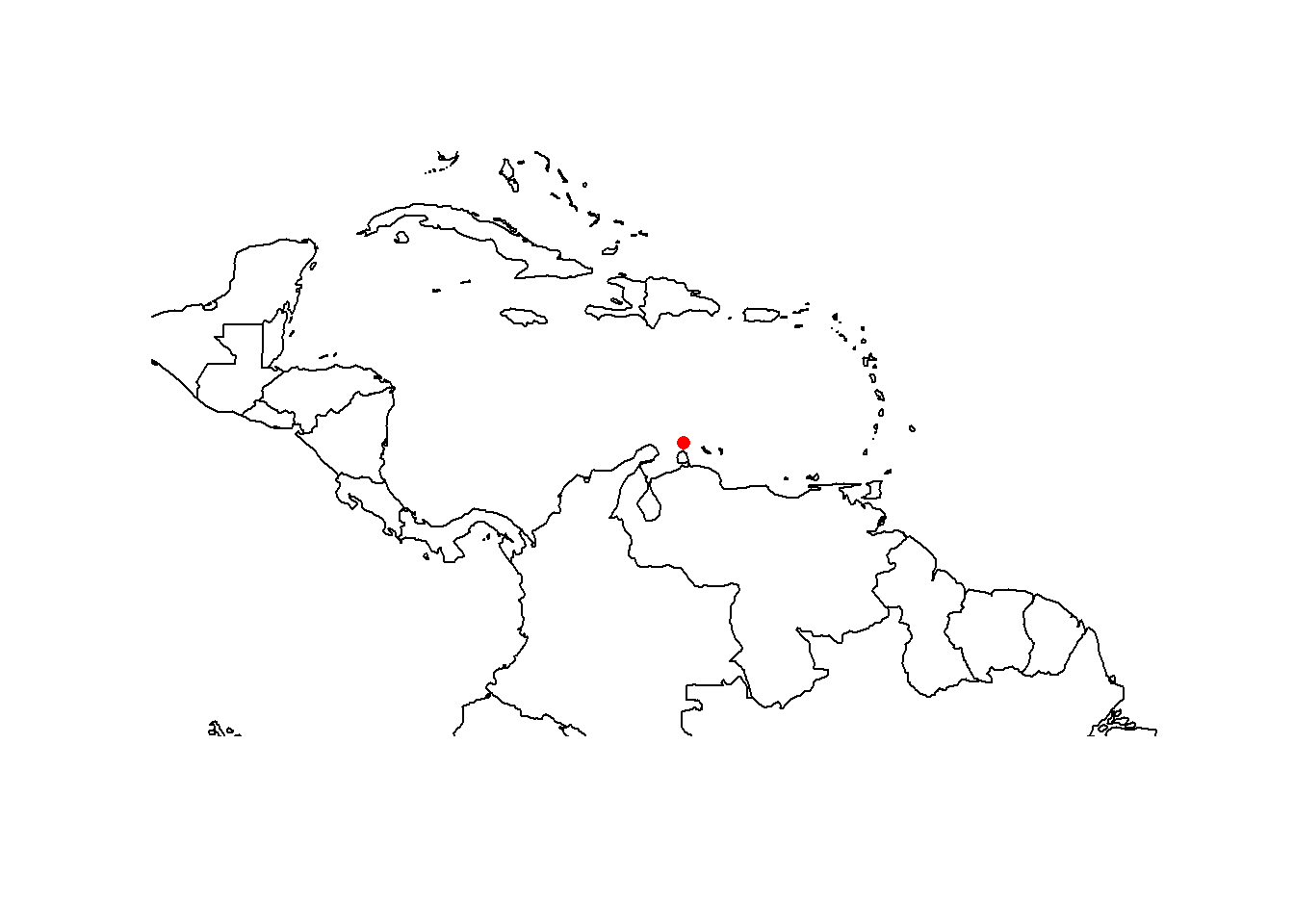

The world map, plotted in native lat-lon decimal degrees, zoomed to level 3, centered on the country of Aruba, and plotted by R’s native `plot` function.

Example 2: Juneau, Alaska

The following code demonstrates that zoomToPoint works in a projected CRS. This code also demonstrates how to compute the extent first, then generate the plot. In this scenario, more plotting options, such as color, are available. But first, a plot of the native United States object in worldmap.

us <- worldmap |> 
  dplyr::filter(grepl("United States", name)) 
plot(us$geometry)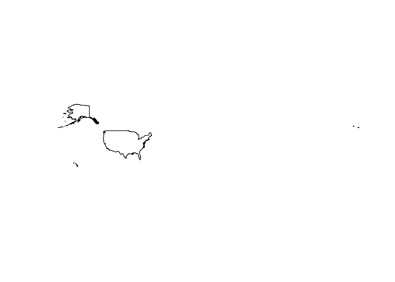

Figure 1: Full extent of the U.S. map object plotted by R’s native `plot` function.

The extent of this plot is too wide to see detail. The next code block projects the us object to a CRS appropriate for Alaska (Alber’s Alaska) and zooms in on the city of Juneau. I used Google Maps to obtain the lat-lon of Juneau.

juneau_ll <- sf::st_sfc(sf::st_point(c( -134.489762, 58.280156)), crs = 4326)
us_3338 <- sf::st_transform(us, 3338) # 3338 = EPSG code for Alber's Alaska
juneau_3338 <- sf::st_transform(juneau_ll, 3338)

ext <- zoomToPoint(juneau_3338, zoomLevel = 4.5)
plot(ext$geometry, border = "wheat")
plot(us_3338$geometry, add=T, col = "wheat3", border = "blue4")
plot(juneau_3338, add=T, col="red", pch=16)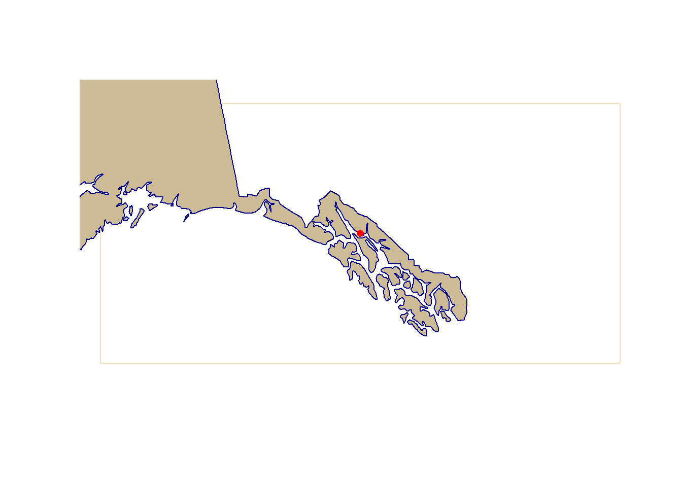

Figure 2: The U.S. map, projected, zoomed to level 4.5, centered on Juneau AK, and plotted by R’s native `plot` function.

As is, the computed extent based on zoomLevel is smaller than the total plot extent because native R plots buffer bounding boxes of spatial objects slightly. R also makes the horizontal and vertical coordinates of the plot equal in real coordinates, so that the map looks right. If the plot’s buffer or real coordinate rectangle is a problem, users can use sf::st_crop to clip x to the extent computed by zoomToPoint. Compare the clipped version (Figure 3) to the unclipped version (Figure 2).

plot(ext$geometry, border = "wheat")
plot(us_3338$geometry |> sf::st_crop(ext), add=T, col = "wheat3", border = "blue4")
plot(juneau_3338, add=T, col="red", pch=16)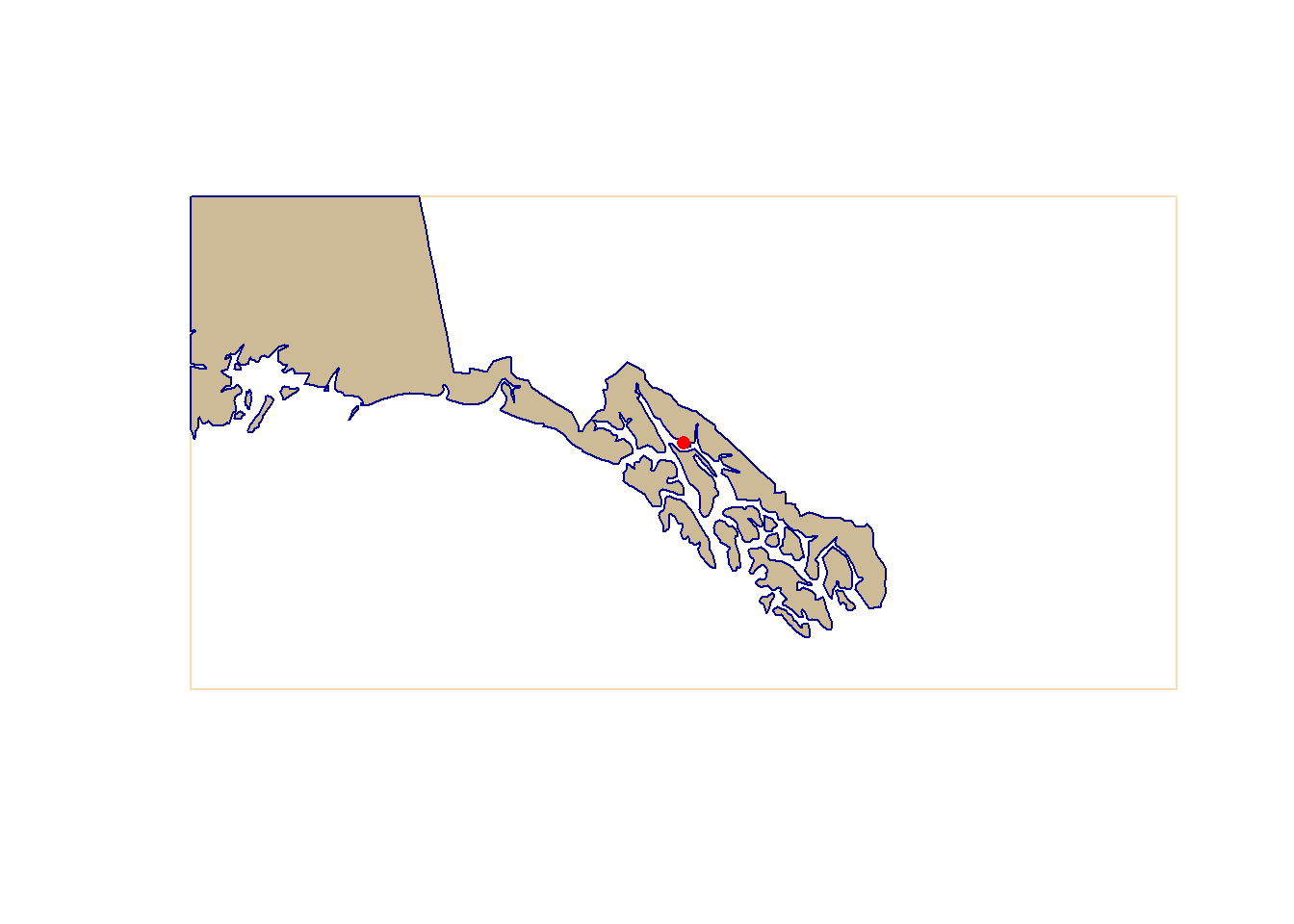

Example 3: ggplot

The extent of ggplot spatial plots is controlled by ggplot2::coord_sf. Min-max coordinates in the extent returned by zoomToPoint can be passed to ggplot2::coord_sf to set the extent of ggplots. First, the full extent of the U.S. object constructed earlier.

ggplt <- ggplot2::ggplot() + 
  ggplot2::geom_sf(data = us_3338) +
  ggplot2::theme_bw()
ggplt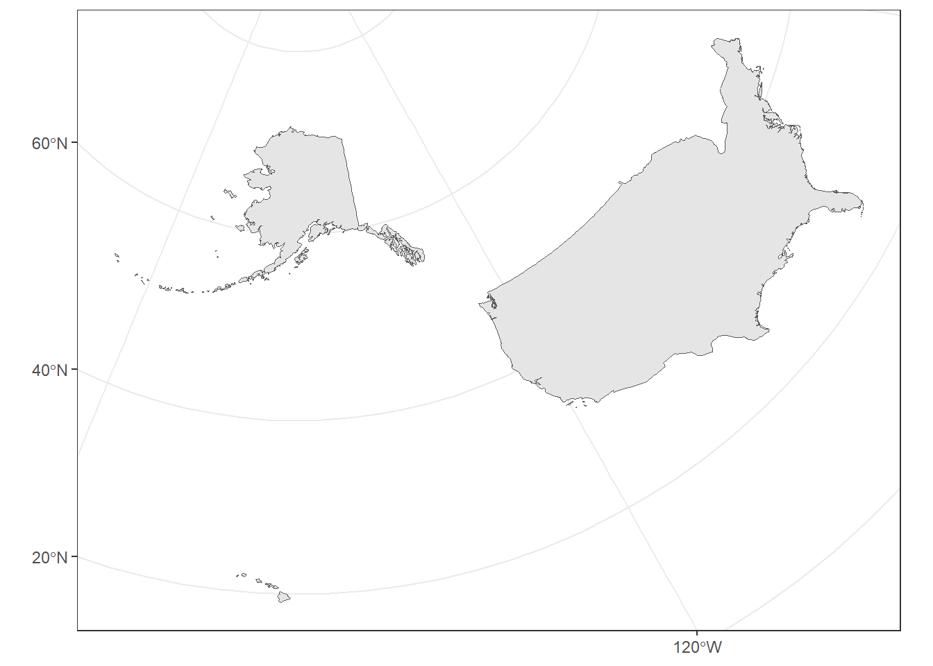

The full extent of the U.S. map object, plotted by `ggplot`.

ggplots of spatial objects are awesome. Note that geom_sf is smart enough to not wrap the Aleutian islands around to the other side of the plot, like plot did (Figure 1). Now, the extent returned by zoomToPoint is used to focus on the area around Juneau AK, similar to (Figure 3).

# coords_sf expects x and y limits, not ll and ur corners
ggplt <- ggplot2::ggplot() + 
  ggplot2::geom_sf(data = us_3338) +
  ggplot2::geom_sf(data = juneau_3338, color = 'red') +
  ggplot2::coord_sf(xlim = range(sf::st_coordinates(ext)[,"X"])
                    , ylim = range(sf::st_coordinates(ext)[,"Y"])) +
  ggplot2::theme_bw()
ggplt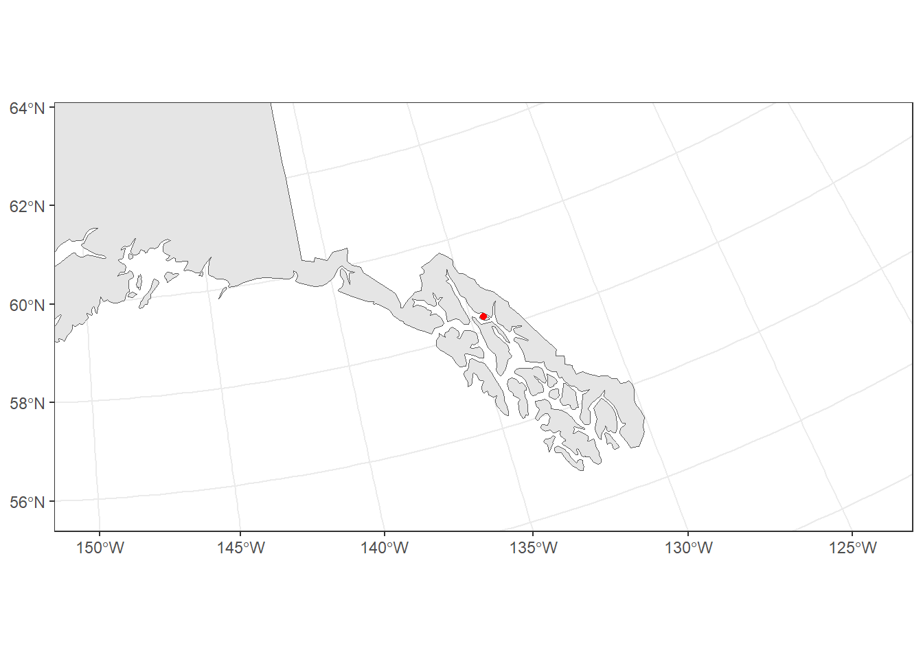

The U.S. map, projected, zoomed to level 4.5, centered on Juneau AK, and plotted by `ggplot`.

Expansions

A more robust version of zoomToPoint would check equality of centerPt’s CRS and x’s CRS, assuming x is present. zoomToPoint could be made to accept center points of different classes. For example, a sf data frame containing POINT geometries could be converted internally to a sfc_POINT using sf::st_as_sfc(). zoomToPoint could also accept any sf object and compute its centroid (e.g., using sf::st_centroid). The plot of x could then be centered on the centroid.

Function Description

Parameters:

Return Value:

Function zoomToPoint

Examples

Example 1: Aruba

Example 2: Juneau, Alaska

Example 3: ggplot

Expansions

Function `zoomToPoint`