Traveling Salesman and BAS

An efficient route through spatially balenced points

Sampling

Author

Trent McDonald

Published

April 26, 2023

In this post, I discuss the practicalities of route finding for spatially balanced samples and demonstrate an efficient route through the set of spatial points.

Background

Everyone knows that spatially balanced samples are the best way to sample space. Multiple algorithms and packages produce spatially balanced samples. The best spatially balanced algorithm in terms of speed and balance is Balanced Acceptance Sampling (BAS) (Robertson et al. (2013)). R package SDraw draws BAS and other types of spatially balanced sample.

But, the following statement always comes up:

If I visit the spatially balanced sample in order, I travel back and forth across the study area and that is way inefficient.

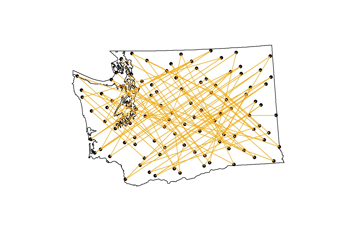
Here is an example. I will draw a BAS sample from the state of Washington and connect sample locations in their BAS order. Strict BAS order “bounces all over” the study area.

library(SDraw)

Loading required package: sp

rgeos version: 0.6-4, (SVN revision 699)
 GEOS runtime version: 3.11.2-CAPI-1.17.2 
 Please note that rgeos will be retired during October 2023,
plan transition to sf or terra functions using GEOS at your earliest convenience.
See https://r-spatial.org/r/2023/05/15/evolution4.html for details.
 GEOS using OverlayNG
 Linking to sp version: 2.1-0 
 Polygon checking: TRUE

SDraw - Sample Draws (v 3.0.0)

data(WA)
basPoints <- SDraw::sdraw(WA, 100, type = "BAS")
plot(WA)
plot(basPoints, add=T, pch=16)
lines(coordinates(basPoints), col = "orange")

# Travel distance in km
(bas_len <- LineLength(coordinates(basPoints)) / 1000)

[1] 25586.2

Strictly speaking, “bouncing all over” is the property that provides good spatial balance to all contiguous sub-samples of the original, and this is a very desirable property statistically. It is not a desirable property if you are trying to reduce costs.

The Loophole

If you know that you will be visiting at least \(n\) locations in the spatially balanced sample, you do not need to visit sample locations in their BAS order. You can visit those \(n\) points in any order. The only danger is that if you eventually fail to visit all \(n\), the spatial balance of the realized sample will be compromised. Even if the realized spatial balance is less than ideal, locations you did visit were still included with equal probability (assuming the original sample was drawn with equal probabilities).

The Traveling Salesperson

Setting aside the fear of not finishing \(n\) locations, we can calculate any visitation schedule we want. The Traveling Salesman Problem (TSP) is a very efficient route and a good choice for determining a route through points in a spatially balanced sample. The TSP attempts to minimize travel distance assuming all points in a set must be visited. Picture a traveling salesperson trying to minimize their driving distance between \(n\) cities. The TSP has a long history in mathematics and several R packages compute a TSP route. In practice, most implementations do not arrive at the absolute shortest path because computation time is too long; but, they get close and that is good enough in the real world. The best TSP route finding R package I have found is TSP and I use their ETSP function (Euclidian traveling salesperson problem).

Example

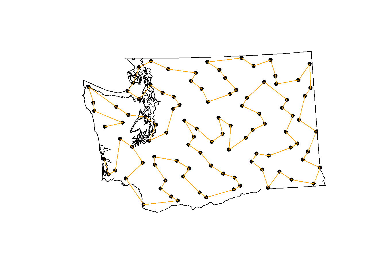
I know I will visit all 100 points in the BAS sample of Washington that I drew earlier. The following code computes the TSP route, constructs a re-ordered sample, plots it, and makes a comparison to length of strict BAS route.

etsp <- TSP::ETSP(coordinates(basPoints))
tour <- TSP::solve_TSP(etsp)
# Route is computed. Now make into spatial object.
tspRoute <- data.frame(basPoints)[drop(as.matrix(tour)),]
tspRoute$tspOrder <- seq(1:nrow(tspRoute))
tspRoute <- sp::SpatialPointsDataFrame(tspRoute[,c("coords.x1","coords.x2")], 
                                     data = tspRoute, 
                                     proj4string = CRS(proj4string(basPoints)))
# Plot
plot(WA)
plot(tspRoute, add=T, pch = 16)
lines(coordinates(tspRoute), col = "orange")

# Travel distance in km
(tsp_len <- LineLength(coordinates(tspRoute)) / 1000)

[1] 4097.383

# Reduction in travel distance (percent)
(pReduced <- abs(bas_len - tsp_len) / bas_len)

[1] 0.8398596

The TSP route is 84% shorter than the BAS route, a savings of 21,489 kilometers.

The final data frame maintains columns for both the BAS and TSP order so it is possible to re-order back to BAS if necessary. Here are the first 10 sample points, with superfluous columns omitted.

(head(data.frame(tspRoute)[, c("sampleID", "tspOrder", "coords.x1", "coords.x2")]))

    sampleID tspOrder coords.x1 coords.x2
189       97        1  421946.7   5178182
45        23        2  434290.8   5138549
153       78        3  450161.8   5148457
57        30        4  462505.9   5227723
129       66        5  492484.4   5207906
81        44        6  518936.1   5168274

Final Comments

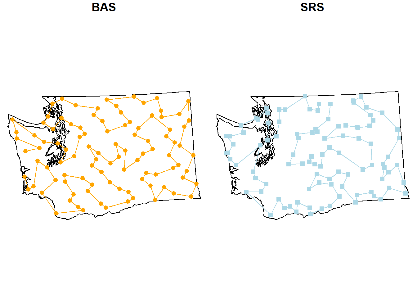
If a researcher is tempted to forgo spatially balanced sampling in favor of simple random sampling (SRS) because they feel simple random sampling yields a more efficient route (is cheaper), they should reconsider. The traveling salesperson route applied to a spatially balanced sample is only slightly higher (5% to 20%) than the traveling salesperson route applied to a simple random sample. The only reason that the SRS route is shorter is that many SRS points are close together, i.e., it is not spatially balanced. In fact, if the SRS sample happens to be spatially balanced, the TSP routes through BAS and SRS points will be nearly identical in length. In the end, I believe that spatial balance of the sample will benefit the study more than not, and that the additional travel costs of the route are well worth it. Here is a comparison for one sample realization:

# Simple random sample of 100 in Washington
srsPoints <- SDraw::sdraw(WA, 100, type = "SRS")
# Compute TSP route
etsp <- TSP::ETSP(coordinates(srsPoints))
tour <- TSP::solve_TSP(etsp)
srsRoute <- data.frame(srsPoints)[drop(as.matrix(tour)),]
srsRoute <- sp::SpatialPointsDataFrame(srsRoute[,c("x","y")], 
   data = srsRoute, 
   proj4string = CRS(proj4string(basPoints)))
(srs_len <- LineLength(coordinates(srsRoute)) / 1000)

[1] 3669.463

(lengs <- c(tspLen_km = tsp_len, srsLen_km = srs_len, pctIncBas = abs(tsp_len - srs_len) / srs_len))

   tspLen_km    srsLen_km    pctIncBas 
4097.3832754 3669.4625076    0.1166167

For this realized sample, the TSP BAS route is 11.7% longer than the TSP SRS route, a increase of 428 kilometers. But, the realized BAS sample has much better spatial balance than the realized SRS, as can be seen in the overlaid plot of TSP through BAS (orange) and TSP through SRS (light blue), below.

par(mfrow=c(1,2), mar=c(0,0,1.1,0))
plot(WA, main = "BAS")
plot(tspRoute, add=T, pch = 16, col = "orange")
lines(coordinates(tspRoute), col = "orange")
plot(WA, main = "SRS")
plot(srsRoute, add=T, pch = 15, col = "lightblue")
lines(coordinates(srsRoute), col = "lightblue")

References

Robertson, Blair. L., J A Brown, Trent L. McDonald, and P Jaksons. 2013. “BAS: Balanced Acceptance Sampling of Natural Resources.” Biometrics 69 (3): 776–84. https://doi.org/10.1111/biom.12059.