Line Transects - No Covariates

Note

This tutorial was rendered using Rdistance version 4.5.0.

Abundance via line-transect distance-sampling when detection does not depend on covariates.

Construct the Rdistance data frame

library(Rdistance)

Loading required package: units

udunits database from C:/Users/trent/AppData/Local/R/win-library/4.6/units/share/udunits/udunits2.xml

Rdistance (v4.5.0)

# Example data (see ?sparrowDetectionData)
data("sparrowDetectionData")  # access example data
data("sparrowSiteData")
head(sparrowDetectionData)  # inspect data

  siteID groupsize sightdist sightangle     dist
1     A1         1        65         15 16.8 [m]
2     A1         1        70         10 12.2 [m]
3     A1         1        25         75 24.1 [m]
4     A1         1        40          5  3.5 [m]
5     A1         1        70         85 69.7 [m]
6     A1         1        10         90 10.0 [m]

head(sparrowSiteData)

  siteID  length observer bare herb shrub height shrubclass
1     A1 500 [m]     obs4 36.7 15.9  20.1   26.4       High
2     A2 500 [m]     obs4 38.7 16.1  19.3   25.0       High
3     A3 500 [m]     obs5 37.7 18.8  19.8   27.0       High
4     A4 500 [m]     obs5 37.7 17.9  19.9   27.1       High
5     B1 500 [m]     obs3 58.5 17.6   5.2   19.6        Low
6     B2 500 [m]     obs3 56.6 18.1   5.2   19.0        Low

# Make nested data frame required by Rdistance
sparrowDf <- RdistDf(sparrowSiteData
                     , sparrowDetectionData
                     , by = "siteID"
                     , pointSurvey = FALSE
                     , observer = "single"
                     , .detectionCol = "detections"
                     , .effortCol = "length")

Inspect the Rdistance data frame.

head(sparrowDf)

# A tibble: 6 × 9
# Rowwise:  siteID
  siteID         detections length observer  bare  herb shrub height shrubclass
  <fct>  <list<tibble[,4]>>    [m] <fct>    <dbl> <dbl> <dbl>  <dbl> <fct>     
1 A1               [15 × 4]    500 obs4      36.7  15.9  20.1   26.4 High      
2 A2               [13 × 4]    500 obs4      38.7  16.1  19.3   25   High      
3 A3               [10 × 4]    500 obs5      37.7  18.8  19.8   27   High      
4 A4               [14 × 4]    500 obs5      37.7  17.9  19.9   27.1 High      
5 B1                [1 × 4]    500 obs3      58.5  17.6   5.2   19.6 Low       
6 B3                [6 × 4]    500 obs1      56.8  18.4   7.5   19.7 Low       

summary(sparrowDf, formula = dist ~ groupsize(groupsize))

Transect type: line
Effort:
       Transects: 72        
    Total length: 36000 [m] 
Distances:
   0 [m] to 207 [m]: 356
Sightings:
         Groups: 356 
    Individuals: 374 

# see detections on transect A1
sparrowDf |> 
  dplyr::filter(siteID == "A1") |>
  dplyr::reframe(detections)

# A tibble: 15 × 5
   siteID groupsize sightdist sightangle dist
   <fct>      <int>     <int>      <int>  [m]
 1 A1             1        65         15 16.8
 2 A1             1        70         10 12.2
 3 A1             1        25         75 24.1
 4 A1             1        40          5  3.5
 5 A1             1        70         85 69.7
 6 A1             1        10         90 10  
 7 A1             1        15         85 14.9
 8 A1             1         5         20  1.7
 9 A1             1         4         90  4  
10 A1             1        10         85 10  
11 A1             1        10         80  9.8
12 A1             1        70         75 67.6
13 A1             1        75         80 73.9
14 A1             1        75         85 74.7
15 A1             1        30         45 21.2

# see detections on 5th transect
sparrowDf$detections[[5]]

# A tibble: 1 × 4
  groupsize sightdist sightangle dist
      <int>     <int>      <int>  [m]
1         1        13         25  5.5

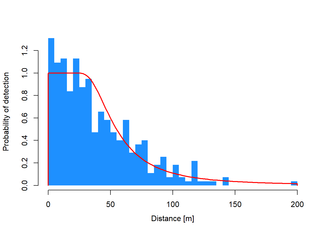
Estimate hazard rate distance function

# First, set upper (right) truncation distance
whi <- set_units(200, "m")

# Fit hazard rate likelihood 
dfuncFit <- sparrowDf |>
  dfuncEstim(dist ~ groupsize(groupsize)
             , likelihood = "hazrate"
             , w.hi = whi)

# plot
plot(dfuncFit
   , nbins = 30
   , col = "dodgerblue"
   , border = NA)

Density and abundance: Point estimates

# First, set study area size or desired density base
oneHectare <- set_units(1, "ha")

# To save computation time, set `ci = NULL`
# to compute point estimates only, i.e., 
abunFit <- dfuncFit |>
  abundEstim(area = oneHectare
             , ci = NULL)

summary(abunFit)

Call: dfuncEstim(data = sparrowDf, dist ~ groupsize(groupsize),
   likelihood = "hazrate", w.hi = whi)
Coefficients:
             Estimate  SE         z          p(>|z|)      
(Intercept)  3.880325  0.1024181  37.887084  4.199822e-314
k            2.966558  0.3724571   7.964833   1.654475e-15

Message: Success; Asymptotic SE's
Function: HAZRATE  
Strip: 0 [m] to 200 [m] 
Effective strip width (ESW): 64.40994 [m] 
Probability of detection: 0.3220497
Scaling: g(0 [m]) = 1
Log likelihood: -1647.79 
AICc: 3299.614

     Surveyed Units: 36000 [m] 
   Individuals seen: 372 in 354 groups 
 Average group size: 1.050847 
   Group size range: 1 to 3 
Density in sampled area: 8.021536e-05 [1/m^2]
Abundance in 10000 [m^2] study area: 0.8021536

# Estimates are stored inside the output object
data.frame(abunFit$estimates)

        id X.Intercept.        k              density abundance avgEffDistance
1 Original     3.880325 2.966558 8.021536e-05 [1/m^2] 0.8021536   64.40994 [m]
  nGroups nSeen avgGroupSize        area surveyedUnits propUnitSurveyed       w
1     354   372     1.050847 10000 [m^2]     36000 [m]                1 200 [m]

Density and abundance: With confidence intervals

# Set `ci =` to desired confidence level
# Set `R =` to number of bootstrap iterations
abunFit <- dfuncFit |>
  abundEstim(area = oneHectare
             , ci = 0.95
             , R = 100)

Creating CPU cluster with 15 cores...done.
Copying data to cores...done.
100 bootstrap iterations estimated run time ~0.03 [min]. Standby...Actual run time: 3.564 [s]

summary(abunFit)

Call: dfuncEstim(data = sparrowDf, dist ~ groupsize(groupsize),
   likelihood = "hazrate", w.hi = whi)
Coefficients:
             Estimate  SE         z          p(>|z|)      
(Intercept)  3.880325  0.1472417  26.353439  4.687165e-153
k            2.966558  0.4825384   6.147818   7.855619e-10

Message: Success; Bootstrap SE's
Function: HAZRATE  
Strip: 0 [m] to 200 [m] 
Effective strip width (ESW): 64.40994 [m] 
Probability of detection: 0.3220497
Scaling: g(0 [m]) = 1
Log likelihood: -1647.79 
AICc: 3299.614

     Surveyed Units: 36000 [m] 
   Individuals seen: 372 in 354 groups 
 Average group size: 1.050847 
   Group size range: 1 to 3 

Density in sampled area: 8.021536e-05 [1/m^2]
                 95% CI: 6.018921e-05 [1/m^2] to 0.0001122096 [1/m^2]

Abundance in 10000 [m^2] study area: 0.8021536
                             95% CI: 0.6018921 to 1.122096

Final density estimate (at the bottom of the output) is 0.8022 sparrows per hectare (95% CI: 0.6019 to 1.1221).

# Note: all bootstrap results are stored inside the output object
head(data.frame(abunFit$B))

             id X.Intercept.        k              density abundance nGroups
1 Bootstrap_001     4.049845 3.337589 6.456699e-05 [1/m^2] 0.6456699     329
2 Bootstrap_016     3.925242 2.918365 8.550106e-05 [1/m^2] 0.8550106     401
3 Bootstrap_031     3.630062 2.463112 9.794644e-05 [1/m^2] 0.9794644     365
4 Bootstrap_046     3.782188 2.765381 9.291347e-05 [1/m^2] 0.9291347     382
5 Bootstrap_061     3.915956 3.116475 8.170822e-05 [1/m^2] 0.8170822     375
6 Bootstrap_076     3.799366 3.007794 7.795544e-05 [1/m^2] 0.7795544     314
  nSeen avgGroupSize        area surveyedUnits propUnitSurveyed       w
1   340     1.033435 10000 [m^2]     36000 [m]                1 200 [m]
2   416     1.037406 10000 [m^2]     36000 [m]                1 200 [m]
3   384     1.052055 10000 [m^2]     36000 [m]                1 200 [m]
4   402     1.052356 10000 [m^2]     36000 [m]                1 200 [m]
5   386     1.029333 10000 [m^2]     36000 [m]                1 200 [m]
6   333     1.060510 10000 [m^2]     36000 [m]                1 200 [m]
  avgEffDistance
1   73.13679 [m]
2   67.57551 [m]
3   54.45153 [m]
4   60.09175 [m]
5   65.61287 [m]
6   59.32877 [m]